Robot Configuration Design
This page explains humanoid robot configuration selection and overall design.
Humanoid Robots
Before discussing configuration choices in detail, let us first look at different kinds of humanoid robots.
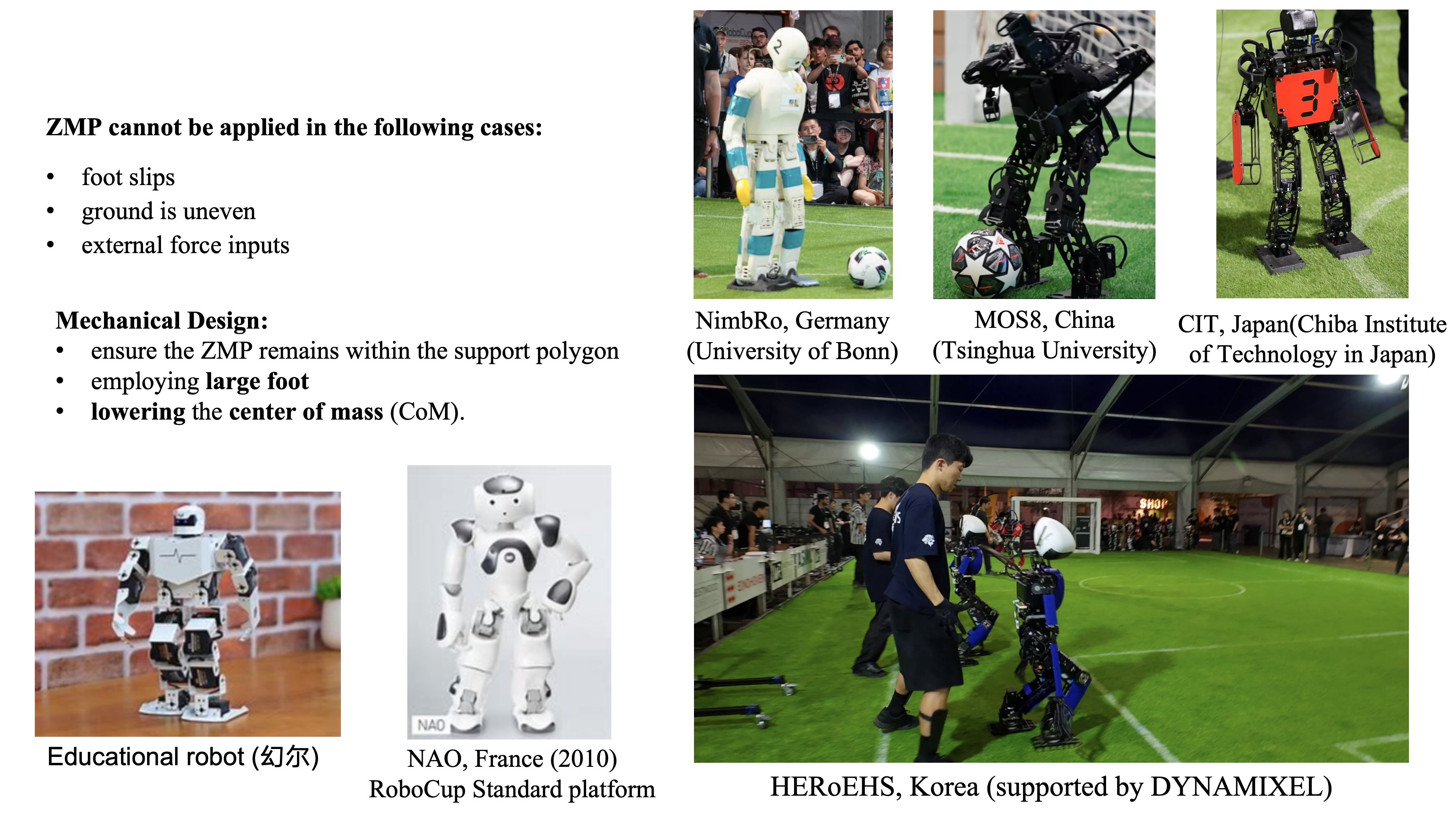
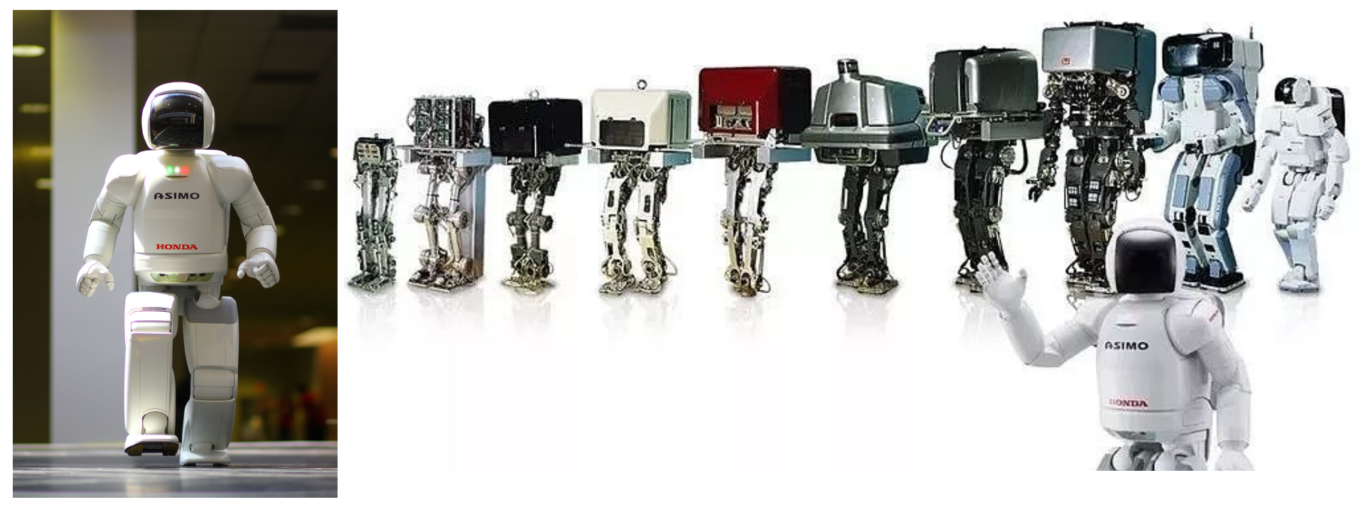
In the first chapter on project background, we introduced several RoboCup robots. In fact, the robots shown there already reflect the characteristics of three eras of humanoid robot development. Broadly speaking, humanoid robots can be divided into three periods, and each era has its representative control algorithm. Before 2015, most humanoid robots used ZMP controllers. Representative examples include NAO, Asimo, and servo-based robots such as MOS8. From 2015 to 2022, optimization-based controllers became dominant, represented by Boston Dynamics Atlas and many robots from the DARPA challenges. From 2023 onward, robots controlled by reinforcement learning have emerged rapidly and their performance continues to improve. A representative example is the Unitree G1.
The ZMP Era
Before 2015, humanoid robots mainly used the ZMP plus linear inverted pendulum model (LIPM) control framework. ZMP, or Zero Moment Point, refers to the point on the sole where, during standing or walking, the resultant moment is zero in all directions except the vertical one if the human or robot is to remain dynamically balanced. By planning gait so that the ZMP always stays within the support region under the foot, stable walking can be achieved.
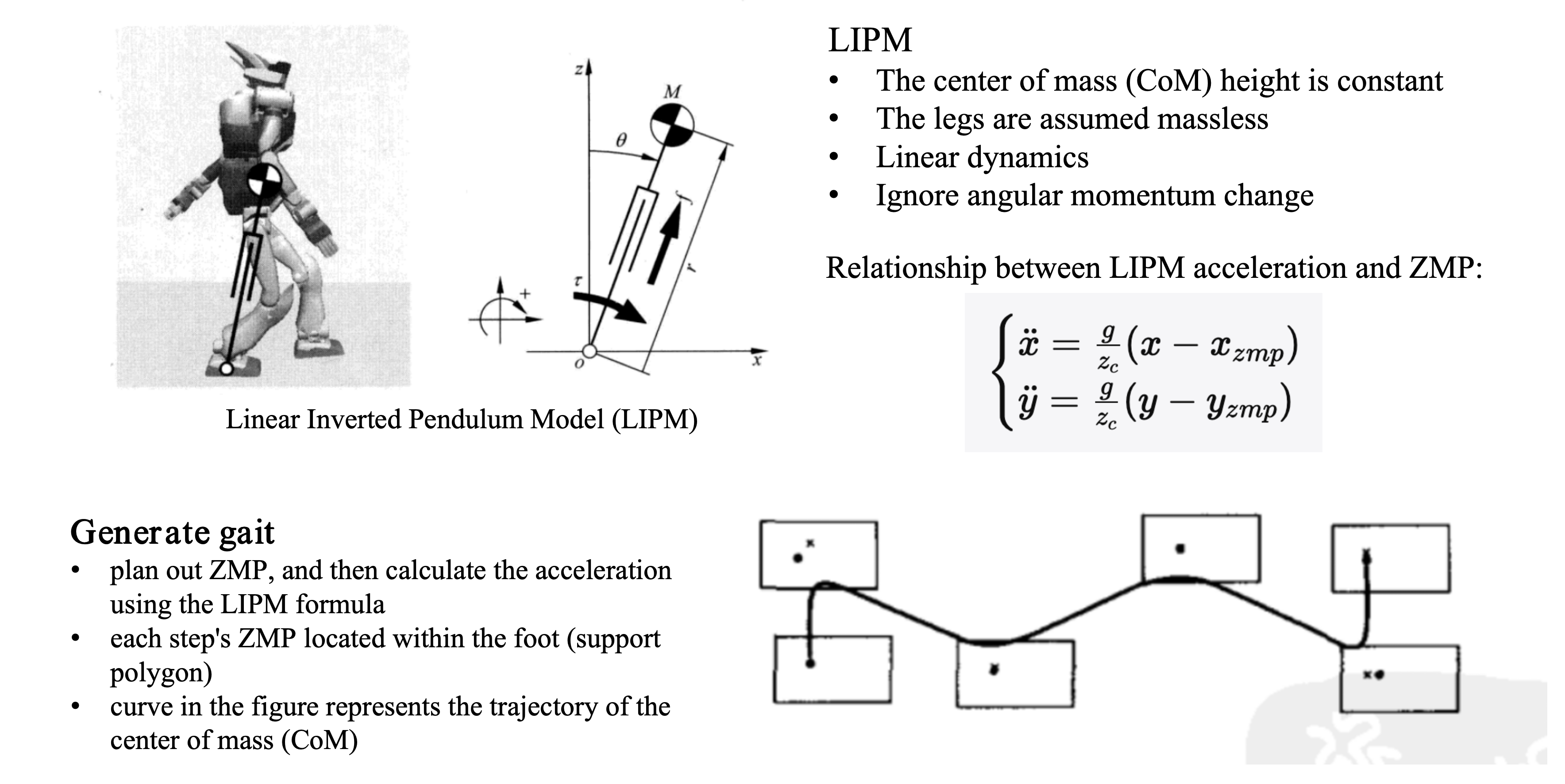
To make it easier for the ZMP to remain inside the support region, robots in this period usually had relatively large feet. The drawback was reduced agility. The limitation of the ZMP method is that it depends on flat and rigid contact surfaces, making it difficult to handle soft, slippery, or complex unknown terrain. Since ZMP-based control does not provide especially strong dynamic performance and most systems relied on position-controlled actuators, servo motors were commonly used during this era.
The Optimization-Control Era
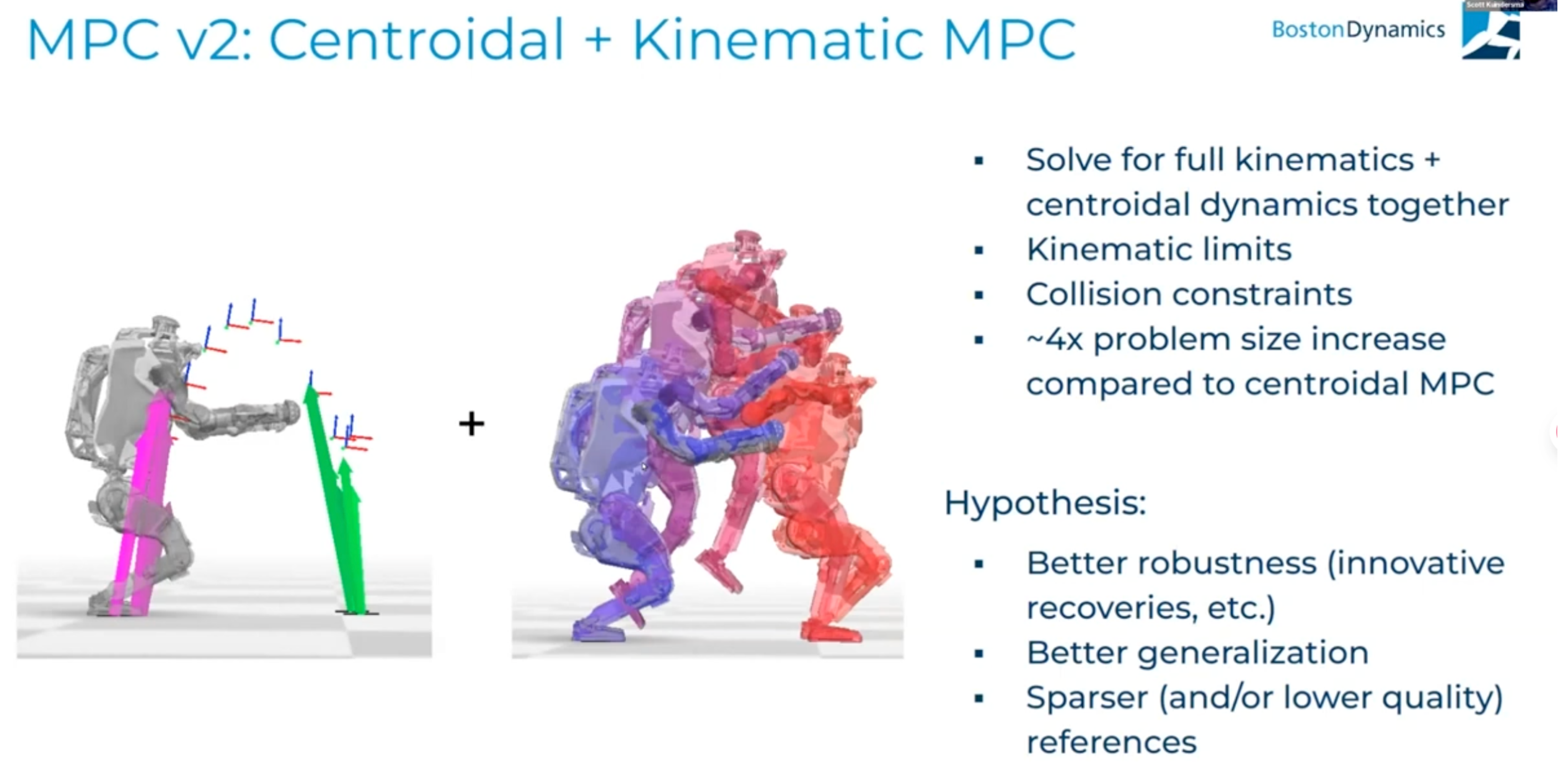
In 2013, Boston Dynamics Atlas appeared and quickly drew global attention. By 2017, Atlas amazed the world with backflips. Atlas used an optimization-based control approach. The core difficulty in optimization control is modeling, because robot dynamics are generally described by complex nonlinear equations. Solving Model Predictive Control (MPC) in a rolling fashion is computationally expensive, so many simplified approaches have been proposed, such as single rigid-body models and simplified whole-body dynamics models. MPC is often used as a planner to compute desired foot contact forces or desired trajectories, followed by a Whole Body Control (WBC) optimizer that computes joint torques under full dynamic constraints. There are many variants of this overall strategy, but the main differences lie in the model choice and in how the optimization problem is formulated and solved.
You can watch a talk explaining the Atlas control strategy on YouTube: Boston Dynamics control talk.
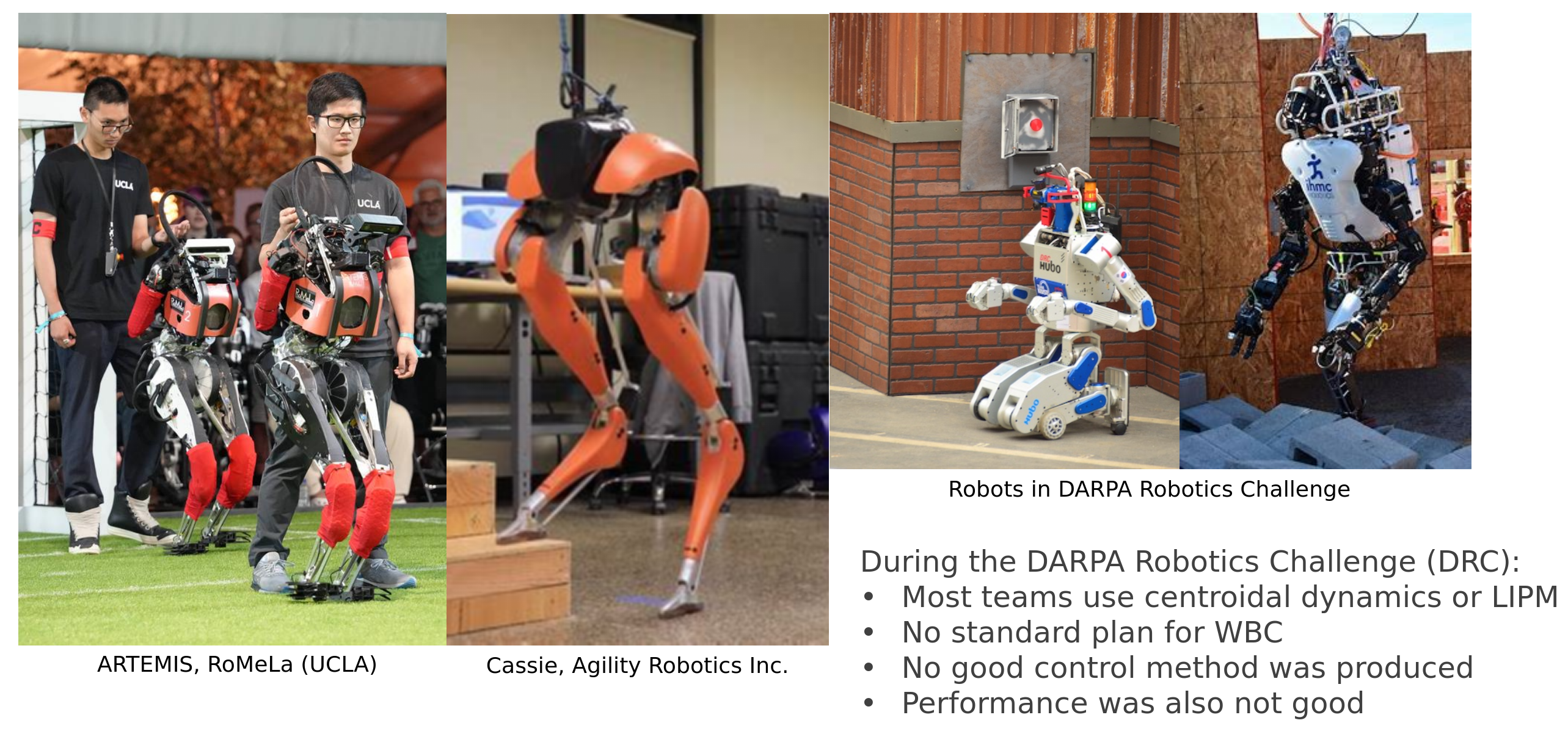
Many robots were developed during this period, such as ARTEMIS from the RoMeLa lab, the Cassie robot, and many robots from the DARPA challenges. These robots differ significantly from earlier ones. For example, some designs place the knee actuator near the hip and connect it to the knee joint through a linkage. The advantage is reduced leg rotational inertia, which improves walking agility. Another advantage is simpler modeling, because leg mass can be neglected in some simplified dynamic models, making the optimization problem easier to solve. In addition, some robots use line-shaped feet because they simplify foot contact constraints and therefore simplify optimization. These features are clearly visible in ARTEMIS and Cassie. Since optimization-based controllers often output joint torques, robots from this period generally use servo motors as actuators.
The Reinforcement Learning Era
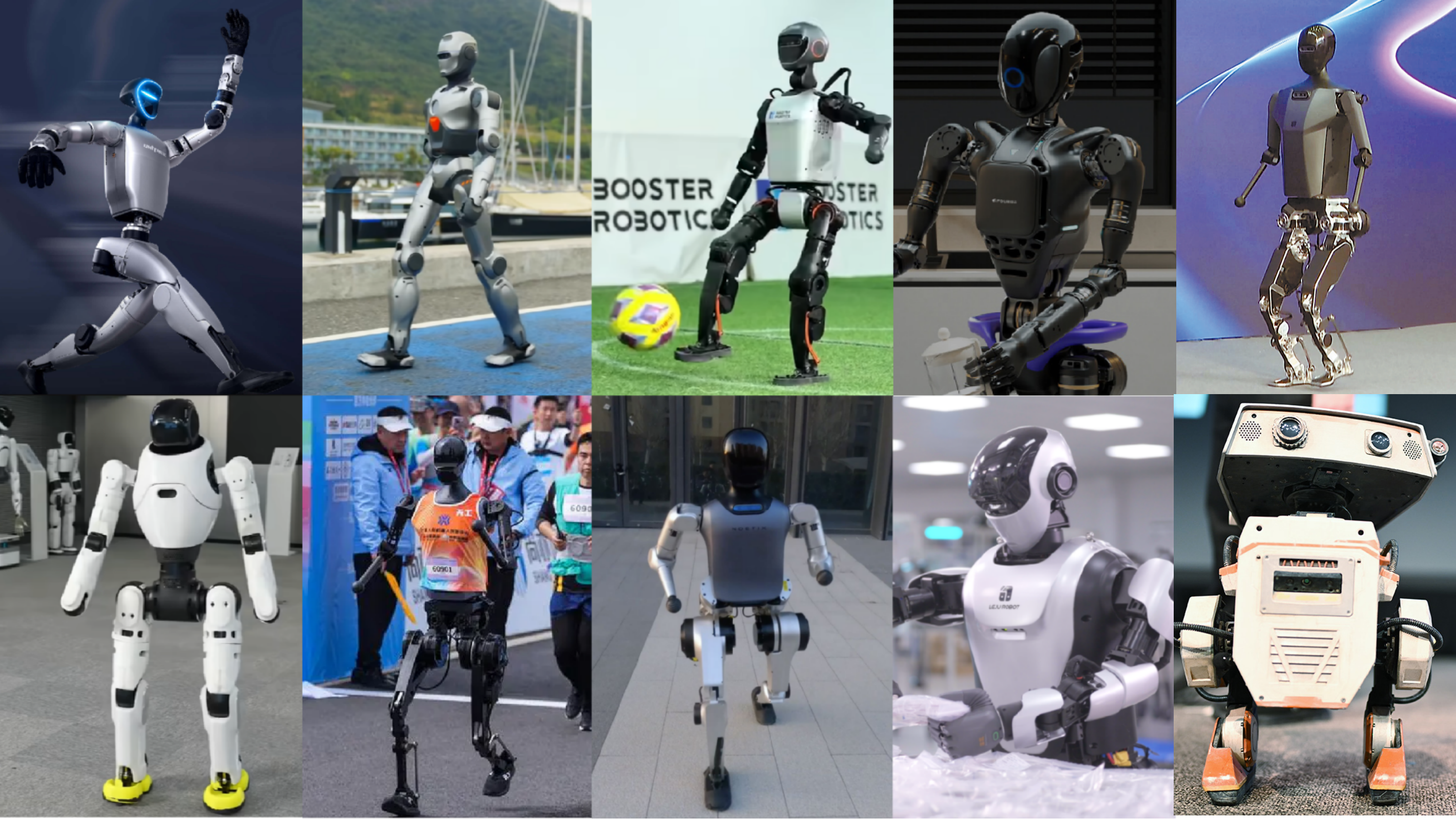
In 2023, reinforcement learning for humanoid robots became increasingly popular, and more and more robots began training inside simulators. In simulation, the full rigid-body dynamics equations are used at every iteration. Through repeated learning in the simulator, the robot can capture the dynamic properties of the complete dynamics model and adapt to different terrains and external disturbances. This helps overcome the limitations of optimization-based approaches, which often rely on simplified dynamic models, cannot observe external forces directly, and cannot naturally incorporate terrain variation. Since robot configuration is no longer constrained by the need for simplified modeling, robots using reinforcement-learning controllers only need to satisfy basic degree-of-freedom requirements. Beyond that, designers focus more on structural stability and joint performance. As for actuators, because the real robot needs to match the dynamic behavior of simulation, the joints generally use servo motors with the same PD position control as in simulation.
Configuration Design
After looking at these robots, it becomes clear that robot body design is closely tied to actuators and control algorithms. As control algorithms evolved from ZMP to optimization control to reinforcement learning, the actuator requirements evolved from servo motors to servo motors with torque control and then to servo motors with position control. Foot design also evolved from large flat feet to line feet to human-like feet. Therefore, the configuration, actuators, and controller need to be considered together from the very beginning of the design process.
MOS9 aims to use a reinforcement-learning controller, so it requires servo motors that support position control. In terms of configuration, like most humanoid robots, it uses a six-degree-of-freedom leg configuration. Since the robot must be able to stand up after falling, the arms need three degrees of freedom. The head must be able to scan the soccer field, so it needs two degrees of freedom.
Leg Configuration
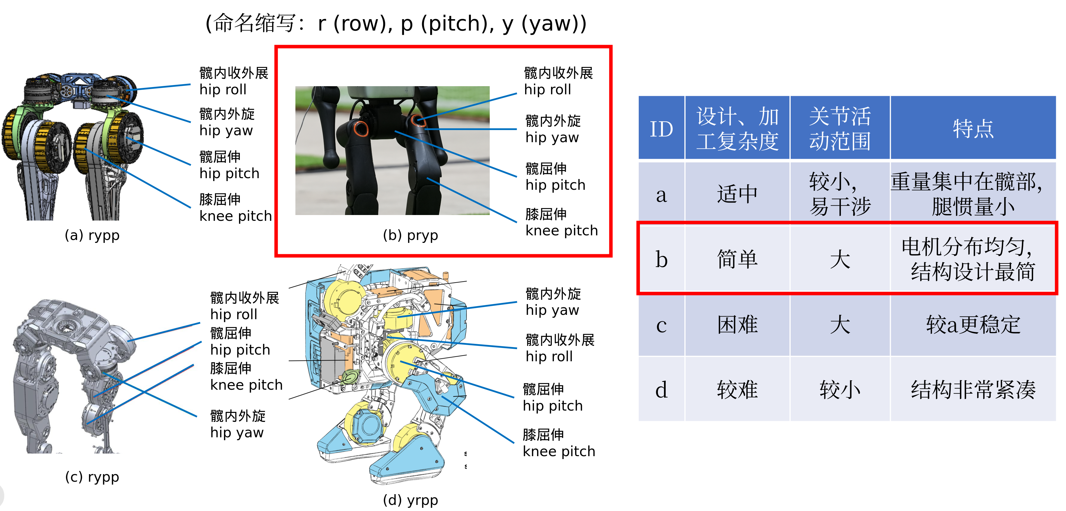
There are several possible thigh configurations, but the differences in degree-of-freedom distribution are usually small. The common choice is three degrees of freedom at the hip, one at the knee, and two at the ankle. A human leg has seven degrees of freedom, with three at the ankle. In practice, however, one fewer degree of freedom at the ankle is usually sufficient, so most robots adopt a six-degree-of-freedom leg design.
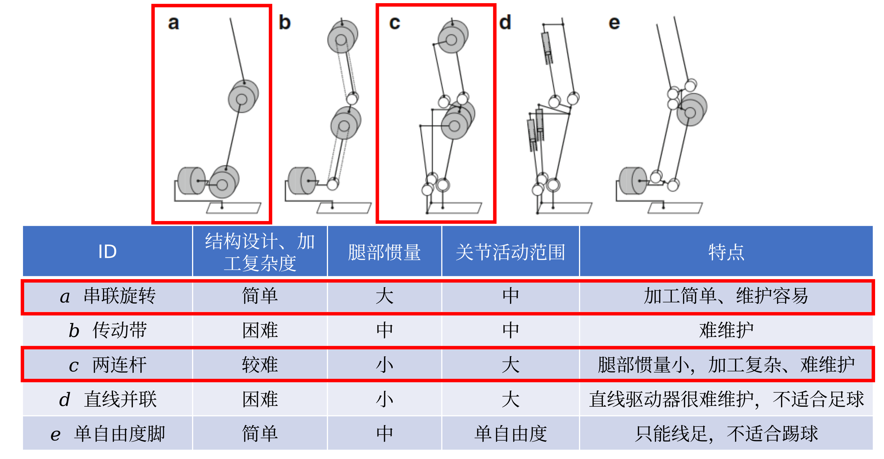
The difference in the three hip degrees of freedom lies in their arrangement, specifically the rotation order of roll, pitch, and yaw. This does not create a major difference in dynamic behavior as long as the joint workspace is suitable. For the knee joint, there are generally two design options. In option (a), the knee actuator is placed near the hip and connected to the knee through a linkage. In option (b), the actuator is mounted directly at the knee. Dynamically, option (a) gives lower leg inertia, but mechanically it introduces more structure. Both are valid choices. If maximum running speed is the goal, option (a) is preferred. For example, the Glory robot, champion of the robot marathon competition, uses this scheme, and Unitree H1 follows a similar idea. If the goal is a balance of overall performance and better stability, option (b) is preferable. MOS9 adopts option (b).
There is also the lower-leg configuration. Many companies adopt configuration (c), mainly because it allows more flexible ankle motion, although it introduces a linkage mechanism. For companies, this added mechanism is not too complex, so performance takes priority. For us, however, simplicity matters more. Configuration (a) makes the ankle look slightly bulkier, but its workspace and dynamic performance are not much worse. In addition, the new Atlas introduced by Boston Dynamics in 2026 also uses this configuration, so configuration (a) is also a well-balanced choice.
Head and Arm Configuration
The head must observe the soccer field, so it needs yaw and pitch degrees of freedom. The arms must support recovery after a fall, so we chose two degrees of freedom at the shoulder and one at the elbow.
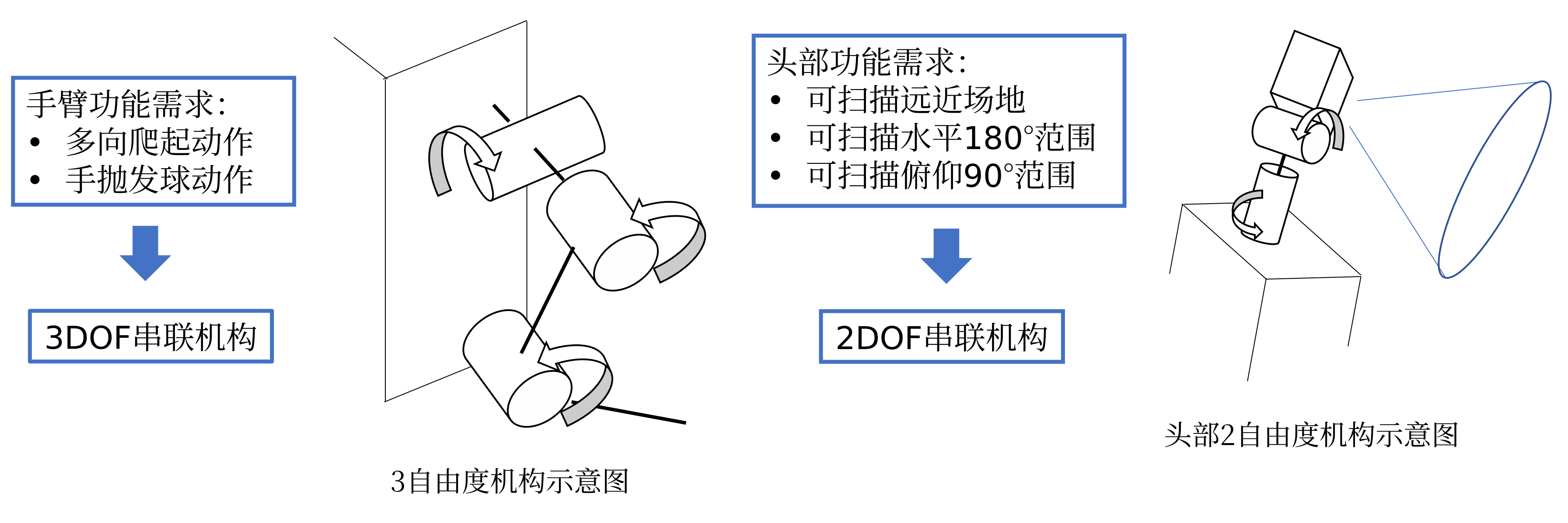
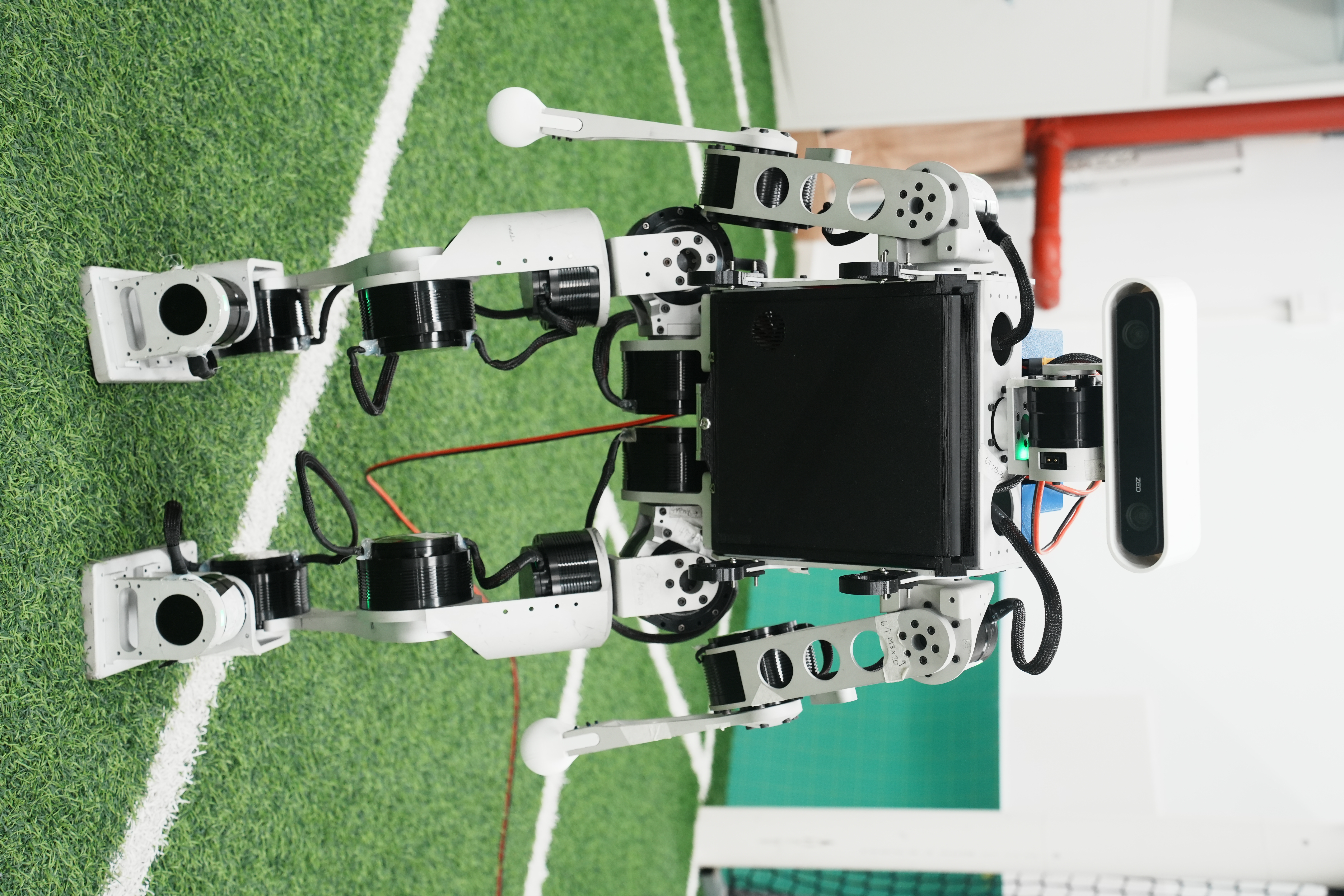
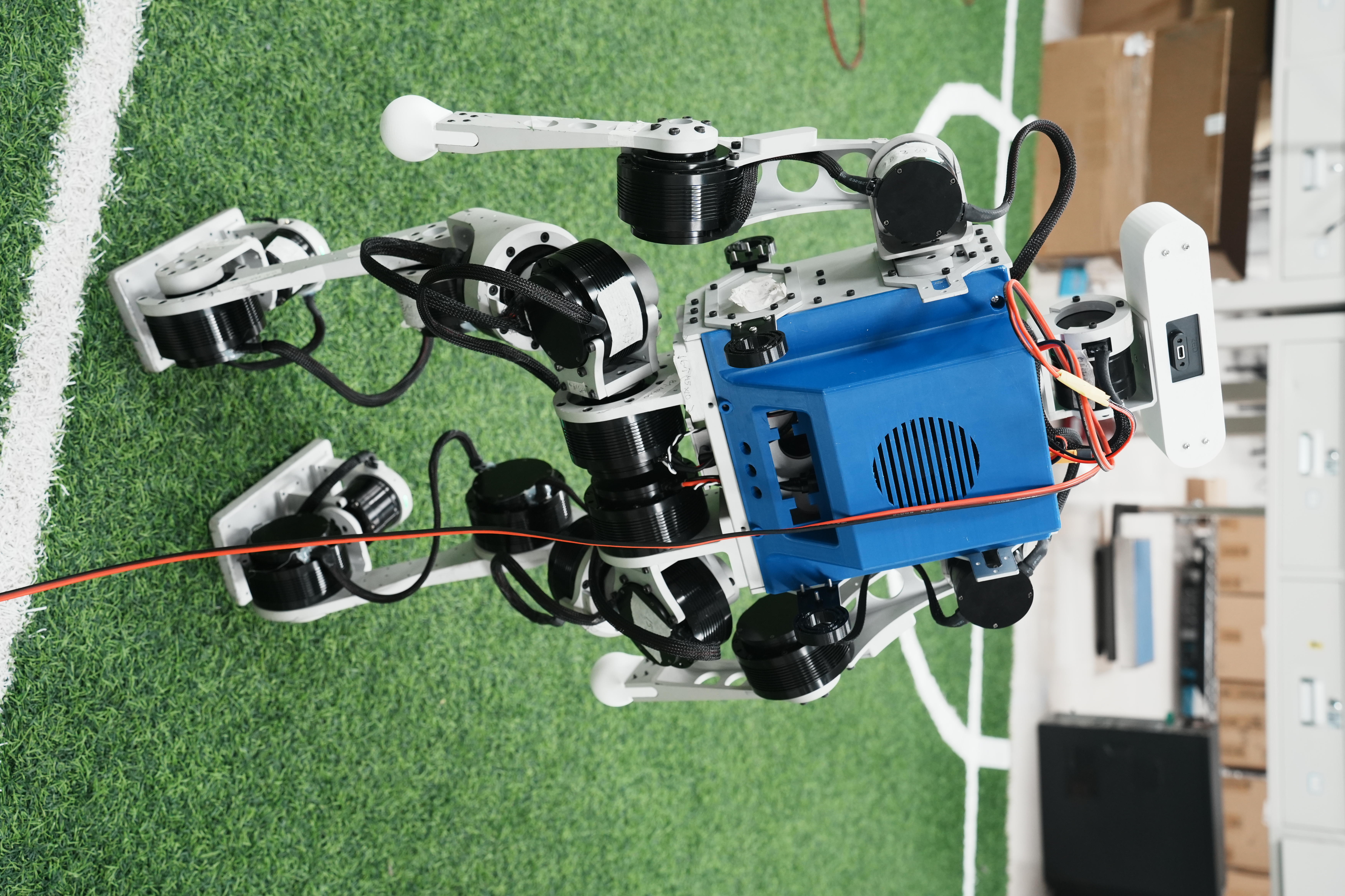
We can now bring back the images of the full robot and observe the degree-of-freedom distribution. You can also examine the many robot images shown earlier to compare how other robots arrange their degrees of freedom.
References
[1]Kajita, Shuuji & Hirukawa, Hirohisa & Harada, Kensuke & Yokoi, Kazuhito. (2014). Introduction to Humanoid Robotics. 10.1007/978-3-642-54536-8.
[2]Ficht, G., & Behnke, S. (2021). Bipedal humanoid hardware design: A technology review. Current Robotics Reports, 2(2), 201-210.