Adversarial Motion Priors (AMP)
This section introduces the robot reinforcement learning algorithm PPO as well as AMP.
PPO
We will not repeat the theoretical details of reinforcement learning here, as there are already many good textbooks. Please refer to other materials for theory study, such as Hands-on Reinforcement Learning. Here we briefly review the PPO formulas.
Let the policy network be \(\pi_\theta(a_t|s_t)\), and the value function be \(V_\phi(s_t)\), where \(s_t\) is the policy observation and \(a_t\) is the policy action. \(\theta\) and \(\phi\) denote the parameters of the policy network and value network, respectively. During training, the policy samples trajectories in the environment and receives immediate rewards, after which it is updated using PPO. Unlike standard PPO, our immediate reward is composed of both the environment task reward and the AMP reward, so the policy update is simultaneously constrained by the task objective and the motion prior.
Let the mixed reward at time step \(t\) be \(r_t\). Then the temporal-difference residual can be written as:
where \(\gamma\) is the discount factor, and \(d_t\) denotes the termination flag. Based on Generalized Advantage Estimation (GAE), the advantage function is computed recursively as:
where \(\lambda\) is the GAE parameter. The return can then be obtained as:
and the advantage is normalized as:
Let the probability ratio between the current policy and the old policy be:
Then the clipped PPO policy objective is written as:
where \(\epsilon\) is the clipping coefficient. The value-function loss is:
where \(V_\phi^{\mathrm{clip}}(s_t)\) denotes the clipped value estimate. In addition, to preserve the policy's exploration capability, an entropy regularization term \(H(\pi_\theta)\) is added to the total loss. Therefore, the optimization objective for the PPO part can be written as:
where \(c_v\) and \(c_e\) are the weight of the value loss and the weight of the entropy regularization term, respectively.
AMP
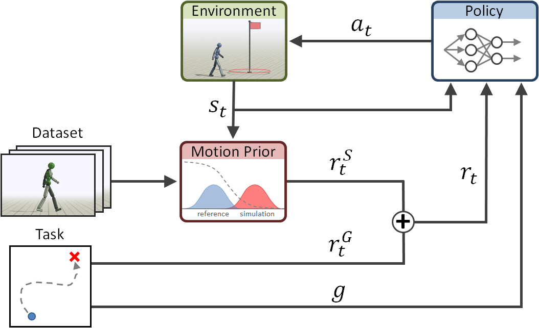
AMP, or Adversarial Motion Priors, essentially introduces a style reward into the reinforcement learning process. In the figure, this is the \(r_t^S\) term, which measures the difference between the robot state \(S_t\) in the simulation environment and the motions in the dataset. By introducing the style reward into the total reward, the robot's motion style is pushed closer to the dataset by increasing the reward value \(r_t^S\). The difference in style is measured using a discriminator, which is a neural network used to measure the difference between two data distributions. Below we explain the formulas for each part of AMP.
AMP Observations and Discriminator Input
AMP does not discriminate directly on the full policy state. Instead, it learns a motion prior in a specially constructed motion-observation space. We define the AMP observation at time step \(t\) as:
where \(q_t\) is the joint position, \(\dot{q}_t\) is the joint velocity, and \(v_t^{\mathrm{body}}\) is the trunk linear velocity in the body frame. To model short-term motion continuity explicitly, we use the transition pair formed by concatenating AMP observations from two adjacent frames as the discriminator input:
Let the discriminator be \(D_\psi(x_t^{\mathrm{amp}})\), where \(\psi\) denotes the discriminator parameters. Then its output is:
This output reflects how consistent the current motion segment is with the reference motion distribution.
AMP Reward Construction
We map the discriminator output into an AMP reward in order to guide the policy toward generating motions that are closer to the expert distribution. The AMP reward is defined as:
where \(w_{\mathrm{amp}}\) is the AMP reward coefficient. When the discriminator output is close to 1, the current motion segment is closer to the expert motion distribution, and the corresponding reward is larger. When the output deviates from 1, the reward decays quadratically and is clipped to remain nonnegative.
Let the original environment task reward be \(r_{\mathrm{task},t}\). Then the mixed reward finally used for the PPO update is written as:
where \(\alpha\) is the interpolation coefficient for the task reward. This mixing method allows the policy to satisfy both the task completion objective and the motion-style constraint during optimization.
Discriminator Supervised Loss
Let the expert sample be:
and the policy sample be:
We train the discriminator using a mean-squared-error form such that it outputs a value close to \(+1\) for expert samples and close to \(-1\) for policy samples. The corresponding losses are:
Therefore, the base discriminator loss is:
Through this loss, the discriminator continually pushes apart the outputs of expert motion and policy motion, while the policy, by maximizing the AMP reward, drives the motion segments it generates toward the expert distribution.
Gradient Penalty and Input Normalization
To improve the stability of adversarial training, we add a gradient-penalty term during discriminator training. Let the expert input be:
Then the gradient penalty is defined as:
where \(\lambda_{\mathrm{gp}}\) is the gradient-penalty coefficient. This term suppresses excessive sensitivity of the discriminator to its inputs and thereby reduces training oscillation.
In addition, to eliminate the influence of state variables with different physical scales on discriminator training, we normalize the AMP input. Let the raw input be \(x\), and the normalized input be \(\hat{x}\). Then:
where \(\mu\) and \(\sigma^2\) are the running mean and variance, respectively, \(\epsilon\) is the numerical stability term, and \(c\) is the clipping threshold. The expert samples and policy samples share the same normalizer so that discrimination is performed on a unified scale.
Joint Optimization Objective
Combining all of the above terms, the overall optimization objective of the training process can be written as:
that is,
Here, the PPO part is responsible for optimizing task performance, the AMP part provides motion-style constraints, and the gradient-penalty term is used to stabilize discriminator training. Through this joint optimization process, the policy can learn more natural, smoother, and more expert-like motion behaviors while still completing control tasks such as velocity tracking.
Simulation Training Results
The training code is open-sourced at: MOS9-AMP.
The final omnidirectional walking results of the robot are shown below. Although the lateral walking may not look especially natural, that is how the retargeted data turned out, and in fact only two data clips were used for the lateral motion.
References
[1] Peng, X. B., Ma, Z., Abbeel, P., Levine, S., & Kanazawa, A. (2021). Amp: Adversarial motion priors for stylized physics-based character control. ACM Transactions on Graphics (ToG), 40(4), 1-20.